It follows from the definition that one can speak of continuity only with respect to those points at which f(x) is defined (no such condition was set when defining the limit of a function). For continuous functions
 , that is, the operations f and lim commute. According to the two definitions of the limit of a function at a point, two definitions of continuity can be given - “in the language of sequences” and “in the language of inequalities” (in the language of ε-δ). It is suggested that you do it yourself.
 For practical use sometimes it is more convenient to define continuity in terms of increments.
The value Δx=x-x 0 is called the increment of the argument, and Δy=f(x)-f(x 0) is the increment of the function when moving from point x 0 to point x.
Definition. Let f(x) be defined at the point x 0 . The function f(x) is called continuous at the point x 0 if an infinitesimal increment of the argument at this point corresponds to an infinitesimal increment of the function, that is, Δy→0 as Δx→0.
Example 1
Prove that the function y=sinx is continuous for any value of x.
Solution.
Let x 0 be an arbitrary point. Giving it an increment Δx, we get the point x=x 0 +Δx. Then ![]()
 . We get
 ![]() .
.
Definition.
The function y=f(x) is called continuous at the point x 0 on the right (left) if
.
A function continuous at an interior point will be both right and left continuous. The converse is also true: if a function is continuous at a point on the left and right, then it will be continuous at that point. However, the function can only be continuous on one side. For example, for 
![]() ,
, ![]() , f(1)=1, therefore, this function is continuous only on the left (for the graph of this function, see Section 5.7.2 above).
, f(1)=1, therefore, this function is continuous only on the left (for the graph of this function, see Section 5.7.2 above).
Definition.
A function is called continuous on some interval if it is continuous at every point of this interval.
In particular, if the interval is a segment , then one-sided continuity is implied at its ends.
Properties of continuous functions
1. All elementary functions are continuous in their domain of definition.2. If f(x) and φ(x), given on some interval, are continuous at the point x 0 of this interval, then the functions will also be continuous at this point.
3. If y=f(x) is continuous at a point x 0 from X, and z=φ(y) is continuous at the corresponding point y 0 =f(x 0) from Y, then the complex function z=φ(f(x )) will be continuous at the point x 0 .
Function breaks and their classification
A sign of the continuity of the function f (x) at the point x 0 is the equality, which implies the presence of three conditions:1) f(x) is defined at the point x 0 ;
2)
 ;
;
3) .
If at least one of these requirements is violated, then x 0 is called the break point of the function. In other words, a discontinuity point is a point where this function is not continuous. From the definition of breakpoints, it follows that the breakpoints of a function are:
a) points belonging to the domain of the function, at which f(x) loses the continuity property,
b) points that do not belong to the domain of f(x), which are adjacent points of two intervals of the domain of the function.
For example, for a function, the point x=0 is a break point, since the function at this point is not defined, and the function
has a discontinuity at the point x=1, which is adjacent for two intervals (-∞,1) and (1,∞) of the domain f(x) and does not exist. The following classification is accepted for discontinuity points.
1) If at the point x 0 there are finite  and
and  , but f(x 0 +0)≠f(x 0 -0), then x 0 is called breaking point of the first kind
, while they call jump function
.
, but f(x 0 +0)≠f(x 0 -0), then x 0 is called breaking point of the first kind
, while they call jump function
.
Example 2
Consider the function 
The break of the function is possible only at the point x=2 (at other points it is continuous like any polynomial).  Let's find
 ![]() ,
, ![]() . Since the one-sided limits are finite, but not equal to each other, at the point x=2 the function has a discontinuity of the first kind. notice, that
. Since the one-sided limits are finite, but not equal to each other, at the point x=2 the function has a discontinuity of the first kind. notice, that ![]() , hence the function is right-continuous at this point (Fig. 2).
, hence the function is right-continuous at this point (Fig. 2).
2) Discontinuity points of the second kind
points are called at which at least one of the one-sided limits is equal to ∞ or does not exist.
 Example 3
The function y=2 1/ x is continuous for all values of x, except for x=0. Find one-sided limits:
Example 3
The function y=2 1/ x is continuous for all values of x, except for x=0. Find one-sided limits: ![]() ,
, ![]() , hence x=0 is a discontinuity point of the second kind (Fig. 3).
, hence x=0 is a discontinuity point of the second kind (Fig. 3).
3) The point x=x 0 is called break point
, if f(x 0 +0)=f(x 0 -0)≠f(x 0).
The gap is “removable” in the sense that it is enough to change (redefine or redefine) the value of the function at this point by setting , and the function will become continuous at the point x 0 .  Example 4
It is known that
Example 4
It is known that  , and this limit does not depend on how x tends to zero. But the function at the point x=0 is not defined. If we extend the definition of the function by setting f(0)=1, then it turns out to be continuous at this point (at other points it is continuous as a quotient of continuous sinx functions and x).
  Example 5
Investigate for continuity a function
Example 5
Investigate for continuity a function  .
.
Solution.
The functions y=x 3 and y=2x are defined and continuous everywhere, including in the indicated intervals. Let's examine the junction point of the gaps x=0: ![]() ,
, ![]() , . We get that , whence it follows that at the point x=0 the function is continuous.
, . We get that , whence it follows that at the point x=0 the function is continuous.
Definition.
A function that is continuous on an interval except for a finite number of discontinuities of the first kind or a removable discontinuity is said to be piecewise continuous on this interval.
Examples of discontinuous functions
 Example 1
The function is defined and continuous on (-∞,+∞) except for the point x=2. Let's define the type of break. Insofar as
Example 1
The function is defined and continuous on (-∞,+∞) except for the point x=2. Let's define the type of break. Insofar as  and
and  , then at the point x=2 there is a discontinuity of the second kind (Fig. 6).
  Example 2
The function is defined and continuous for all x except x=0, where the denominator zero. Let's find one-sided limits at the point x=0:
Example 2
The function is defined and continuous for all x except x=0, where the denominator zero. Let's find one-sided limits at the point x=0: The one-sided limits are finite and different, therefore, x=0 is a discontinuity point of the first kind (Fig. 7).
 Example 3
Determine at what points and what kind of discontinuities the function has
Example 3
Determine at what points and what kind of discontinuities the function has 
This function is defined on [-2,2]. Since x 2 and 1/x are continuous, respectively, in the intervals [-2,0] and , the gap can only be at the junction of the intervals, that is, at the point x=0. Since , then x=0 is a discontinuity point of the second kind.
Example 4
Is it possible to eliminate breaks in functions:
a) at the point x=2;
b)  at the point x=2;
v)  at the point x=1?
Solution.
About example a), we can immediately say that the discontinuity f(x) at the point x=2 cannot be eliminated, since there are infinite one-sided limits at this point (see example 1).
b) The function g(x) although has finite one-sided limits at the point x=2
(![]() ,
,![]() ),
),
but they do not match, so the gap cannot be closed either.
c) The function φ(x) at the discontinuity point x=1 has equal one-sided finite limits: . Therefore, the gap can be eliminated by redefining the function at the point x=1 by putting f(1)=1 instead of f(1)=2.
Example 5 Show that the Dirichlet function

discontinuous at every point on the numerical axis.
Solution. Let x 0 be any point from (-∞,+∞). In any of its neighborhoods, there are both rational and irrational points. This means that in any neighborhood x 0 the function will have values equal to 0 and 1. In this case, there cannot be a limit of the function at the point x 0 either on the left or on the right, which means that the Dirichlet function at each point of the real axis has discontinuities of the second kind.
Example 6 Find function break points

and determine their type.
Solution. Points suspected of breaking are points x 1 =2, x 2 =5, x 3 =3.
At the point x 1 =2 f(x) has a discontinuity of the second kind, since
.
The point x 2 =5 is a point of continuity, since the value of the function at this point and in its vicinity is determined by the second line, not the first: .
Let's explore the point x 3 =3: ,
For independent decision.
Investigate functions for continuity and determine the type of discontinuity points:
1)  ; Answer: x=-1 – break point;
2)  ; Answer: Discontinuity of the second kind at the point x=8;
3)  ; Answer: Discontinuity of the first kind at x=1;
4) 
Answer: At the point x 1 \u003d -5 there is a removable gap, at x 2 \u003d 1 - a gap of the second kind and at the point x 3 \u003d 0 - a gap of the first kind.
5) How should the number A be chosen so that the function 
would be continuous at the point x=0?
Answer: A=2.
6) Is it possible to choose the number A so that the function 
would be continuous at the point x=2?
Answer: no.
Continuity of a function on an interval
| Parameter name | Meaning |
| Article subject: | Continuity of a function on an interval |
| Rubric (thematic category) | Mathematics |
Definition. A function is called continuous on an interval if it is continuous at every point of this interval.
If the function is defined for X=a and wherein f(X) = f(a),
then they say that f(X) at the point and continuous on the right. Similarly, if f(X) = f(b), then we say that at the point b this function left continuous.
Definition. The function is usually called continuous on the segment [ a, b], if it is continuous at each of its points (at the point a continuous on the right, at a point b is continuous on the left).
highest value functions at = f(x) on the segment [ a, b f(x 1) that f(x) £ f(x 1) for everyone X Î [ a, b].
Lowest value functions at = f(x) on the segment [ a, b] it is customary to call such its value f(x 2) that f(x) ³ f(x 2) for everyone X Î [ a, b].
Functions that are continuous on an interval have a number of important properties, which are expressed by the following theorems.
Theorem 3.3.1. A function continuous on the segment [ a, b], reaches its minimum value on it m and the greatest value M, that is, there are such points x 1 and x 2 of this segment, which f(x 1) = m, f(x 2) = M.
The theorem has a simple geometric meaning (see Fig. 2).
 |
Theorem 3.3.2. In case the function at = f(x) is continuous on the interval [ a, b] and takes unequal values at its ends f(a) = A, f(b) = B, A ¹ B, then whatever the number C between A and B, there is a point With Î [ a, b] such that f(With) = C.
The geometric meaning of the theorem is illustrated in Fig.3. Any straight line at= C, where A< C < B (или A >C > B), intersects the graph of the function at = f(x).
Consequence. If the function is continuous on a segment and takes values of different signs at its ends, then there is at least one point on this segment at which the function vanishes.
The geometric meaning of the consequence is illustrated in Fig.4.

Questions for self-control
1. What function is called continuous at a point?
2. Give one more equivalent definition through the increment of a function and arguments.
3. What can be said about the sum, difference, product and quotient of two continuous functions?
4. For what values of the argument are the entire rational and fractional-rational functions continuous?
5. When is a complex function continuous at a point?
6. What is commonly called the breaking point of functions?
7. What points are called discontinuity points of the first kind?
8. What value is usually called the function jump?
9. Explain the concepts of "removable break point". Give examples.
10. What points are called discontinuity points of the second kind? Give examples.
11. Explain the concepts: ""continuity on the interval"", ""continuity on the right"", ""continuity on the left"", ""continuity on the segment"".
12. Define the largest and smallest values of functions.
13. Formulate a theorem on the relationship of continuity on a segment with the largest and smallest values of the function. Explain it with a picture.
14. Formulate a theorem on the connection between the continuity of functions on a segment and the segment of function values. Illustrate its geometric meaning in the figure.
15. Give a consequence of the above theorem and its geometric interpretation.
LECTURE №4
Lecture topic: Function derivative
Lecture plan: The concept of a derivative, its geometric and physical meaning. Basic rules of differentiation. Derivative complex function. Some applications of the derivative.
4.1. The concept of a derivative, its geometric and physical meaning
Consider the function at = f(x) specified in the interval ] a, b[. Let XÎ ] a, b[ and X Î ] a, b[, then the function increment at the point X 0 is expressed by the formula D at = f(x 0+D X) – f(x 0).
Definition. The derivative of the function y = f(x) at the point X 0 is usually called the limit of the ratio of the increment of this function to the increment of the argument when the latter tends to zero:
f'(x 0) = ![]() or y"(x 0) =.
or y"(x 0) =.
The geometric meaning of the derivative: the derivative of this function at a point is equal to the tangent of the angle between the Ox axis and the tangent to the graph of this function at the corresponding point (see Fig. 1):
f"(x 0) = tan a.
In this lesson, we will learn how to establish the continuity of a function. We will do this with the help of limits, moreover, one-sided - right and left, which are not at all scary, despite the fact that they are written as and .
But what is the continuity of a function in general? Until we get to a strict definition, the easiest way to imagine a line that can be drawn without lifting the pencil from the paper. If such a line is drawn, then it is continuous. This line is the graph of a continuous function.
Graphically, a function is continuous at a point if its graph does not "break" at that point. The graph of such a continuous function is ![]() shown in the figure below.
shown in the figure below.

Definition of the continuity of a function through the limit. A function is continuous at a point under three conditions:
1. The function is defined at the point .
If at least one of the above conditions is not met, the function is not continuous at a point. At the same time, they say that the function suffers a break, and the points on the graph at which the graph is interrupted are called the break points of the function. The graph of such a function, which suffers a break at the point x=2, is shown in the figure below.

Example 1 Function f(x) is defined as follows:

Will this function be continuous at each of the boundary points of its branches, that is, at the points x = 0 , x = 1 , x = 3 ?
Solution. We check all three conditions for the continuity of the function at each boundary point. The first condition is met because function defined at each of the boundary points follows from the definition of the function. It remains to check the remaining two conditions.
Dot x= 0 . Find the left-hand limit at this point:
![]() .
.
Let's find the right-hand limit:
x= 0 must be found at the branch of the function that includes this point, that is, the second branch. We find them:
As you can see, the limit of the function and the value of the function at the point x= 0 are equal. Therefore, the function is continuous at the point x = 0 .
Dot x= 1 . Find the left-hand limit at this point:
Let's find the right-hand limit:

Function limit and function value at a point x= 1 must be found at the branch of the function that includes this point, that is, the second branch. We find them:
 .
.
Function limit and function value at a point x= 1 are equal. Therefore, the function is continuous at the point x = 1 .
Dot x= 3 . Find the left-hand limit at this point:
Let's find the right-hand limit:

Function limit and function value at a point x= 3 must be found at the branch of the function that includes this point, that is, the second branch. We find them:
 .
.
Function limit and function value at a point x= 3 are equal. Therefore, the function is continuous at the point x = 3 .
Main conclusion: this function is continuous at every boundary point.
Establish the continuity of a function at a point yourself, and then see the solution
A continuous change in a function can be defined as a change that is gradual, without jumps, in which a small change in the argument entails a small change in the function .
Let's illustrate this continuous change of function with an example.

Let a load hang on a thread above the table. Under the action of this load, the thread is stretched, so the distance l load from the point of suspension of the thread is a function of the mass of the load m, that is l = f(m) , m≥0 .
If we slightly change the mass of the load, then the distance l little change: little change m correspond to small changes l. However, if the mass of the load is close to the tensile strength of the thread, then a small increase in the mass of the load can cause the thread to break: the distance l will increase abruptly and become equal to the distance from the suspension point to the table surface. Function Graph l = f(m) shown in the figure. On the site, this graph is a continuous (solid) line, and at the point it is interrupted. The result is a graph consisting of two branches. At all points except , the function l = f(m) is continuous, and at a point it has a discontinuity.
The study of a function for continuity can be both an independent task and one of the stages of a complete study of the function and the construction of its graph.
Continuity of a function on an interval
Let the function y = f(x) defined in the interval ] a, b[ and is continuous at every point of this interval. Then it is called continuous in the interval ] a, b[ . The concept of continuity of a function on intervals of the form ]- ∞ is defined similarly, b[ , ]a, + ∞[ , ]- ∞, + ∞[ . Now let the function y = f(x) defined on the interval [ a, b] . The difference between an interval and a segment is that the boundary points of the interval are not included in the interval, but the boundary points of the segment are included in the segment. Here we should mention the so-called one-sided continuity: at the point a, staying on the interval [ a, b] , we can only approach from the right, and to the point b- only on the left. The function is called continuous on the interval [ a, b] , if it is continuous at all interior points of this segment, continuous on the right at the point a and left continuous at the point b.
Any of the elementary functions can serve as an example of a continuous function. Every elementary function is continuous on any segment on which it is defined. For example, the functions and are continuous on any interval [ a, b] , the function is continuous on the interval [ 0 , b] , the function is continuous on any segment that does not contain a point a = 2 .
Example 4 Investigate the function for continuity.
Solution. Let's check the first condition. The function is not defined at points - 3 and 3. At least one of the conditions for the continuity of the function on the entire number line is not satisfied. Therefore, this function is continuous on the intervals
.Example 5 Determine at what value of the parameter a continuous throughout domains function 
Solution.
Let's find the right-hand limit for:
![]() .
.
It is obvious that the value at the point x= 2 must be equal ax :
![]()
a = 1,5 .
Example 6 Determine at what values of the parameters a and b continuous throughout domains function 
Solution.
Find the left-hand limit of the function at the point :
![]() .
.
Therefore, the value at the point must be equal to 1:
Let's find the left-side function at the point :
Obviously, the value of the function at the point should be equal to:
Answer: the function is continuous over the entire domain of definition for a = 1; b = -3 .
Basic properties of continuous functions
Mathematics came to the concept of a continuous function by studying, first of all, various laws of motion. Space and time are endless and dependency like paths s from time t, expressed by law s = f(t) , gives an example of a continuous functions f(t) . The temperature of the heated water also changes continuously, it is also a continuous function of time: T = f(t) .
V mathematical analysis some properties possessed by continuous functions are proved. We present the most important of these properties.
1. If a function that is continuous on an interval takes on values of different signs at the ends of the interval, then at some point of this segment it takes on a value equal to zero. More formally, this property is given in a theorem known as the first Bolzano-Cauchy theorem.
2. Function f(x) , continuous on the interval [ a, b] , takes all intermediate values between the values at the endpoints, that is, between f(a) and f(b) . More formally, this property is given in a theorem known as the second Bolzano-Cauchy theorem.
PROPERTIES OF FUNCTIONS CONTINUOUS ON A INTERVAL
Let us consider some properties of functions continuous on an interval. We present these properties without proof.
Function y = f(x) called continuous on the segment [a, b], if it is continuous at all internal points of this segment, and at its ends, i.e. at points a and b, is continuous on the right and left, respectively.
Theorem 1. A function continuous on the segment [ a, b], at least at one point of this segment takes the largest value and at least at one point - the smallest.
The theorem states that if the function y = f(x) continuous on the segment [ a, b], then there is at least one point x 1 Î [ a, b] such that the value of the function f(x) at this point will be the largest of all its values on this segment: f(x1) ≥ f(x). Similarly, there is such a point x2, in which the value of the function will be the smallest of all values on the segment: f(x 1) ≤ f(x).
It is clear that there can be several such points, for example, the figure shows that the function f(x) takes the smallest value at two points x2 and x 2 ".
Comment. The statement of the theorem can become false if we consider the value of the function on the interval ( a, b). Indeed, if we consider the function y=x on (0, 2), then it is continuous on this interval, but does not reach its maximum or minimum values in it: it reaches these values at the ends of the interval, but the ends do not belong to our region.
Also, the theorem ceases to be true for discontinuous functions. Give an example.
Consequence. If the function f(x) continuous on [ a, b], then it is bounded on this interval.
Theorem 2. Let the function y = f(x) continuous on the segment [ a, b] and takes on values of different signs at the ends of this segment, then there is at least one point inside the segment x=C, where the function vanishes: f(C)= 0, where a< C< b

This theorem has a simple geometric meaning: if the points of the graph of a continuous function y = f(x), corresponding to the ends of the segment [ a, b] lie on different sides off axis Ox, then this graph at least at one point of the segment intersects the axis Ox. Discontinuous functions may not have this property.
This theorem admits the following generalization.
Theorem 3 (theorem on intermediate values). Let the function y = f(x) continuous on the segment [ a, b] and f(a) = A, f(b) = B. Then for any number C between A and B, there is such a point inside this segment CÎ [ a, b], what f(c) = C.

This theorem is geometrically obvious. Consider the graph of the function y = f(x). Let f(a) = A, f(b) = B. Then any line y=C, where C- any number between A and B, intersects the graph of the function at least at one point. The abscissa of the intersection point will be that value x=C, at which f(c) = C.
Thus, a continuous function, passing from one of its values to another, necessarily passes through all intermediate values. In particular:
Consequence. If the function y = f(x) is continuous on some interval and takes on the largest and smallest values, then on this interval it takes, at least once, any value between its smallest and largest values.
DERIVATIVE AND ITS APPLICATIONS. DERIVATIVE DEFINITION
Let's have some function y=f(x), defined on some interval. For each argument value x from this interval the function y=f(x) has a certain meaning.
Consider two argument values: initial x 0 and new x.

Difference x–x 0 is called increment of argument x at the point x 0 and denoted Δx. In this way, ∆x = x – x 0 (argument increment can be either positive or negative). From this equality it follows that x=x 0 +Δx, i.e. the initial value of the variable has received some increment. Then, if at the point x 0 function value was f(x 0 ), then at the new point x the function will take the value f(x) = f(x 0 +∆x).
Difference y-y 0 = f(x) – f(x 0 ) called function increment y = f(x) at the point x 0 and is denoted by the symbol Δy. In this way,
| Δy = f(x) – f(x 0 ) = f(x 0 +Δx) - f(x 0 ) . | (1) |
Usually the initial value of the argument x 0 is considered fixed and the new value x- variable. Then y 0 = f(x 0 ) turns out to be constant and y = f(x)- variable. increments Δy and Δx will also be variables and formula (1) shows that Dy is a function of the variable Δx.
Compose the ratio of the increment of the function to the increment of the argument
Let us find the limit of this relation at Δx→0. If this limit exists, then it is called the derivative of this function. f(x) at the point x 0 and denote f "(x 0). So,
derivative this function y = f(x) at the point x 0 is called the limit of the increment ratio of the function Δ y to the increment of the argument Δ x when the latter arbitrarily tends to zero.
Note that for the same function the derivative at different points x can take on different values, i.e. the derivative can be thought of as a function of the argument x. This function is denoted f "(x)
The derivative is denoted by the symbols f "(x),y", . The specific value of the derivative at x = a denoted f "(a) or y "| x=a.
The operation of finding the derivative of a function f(x) is called the differentiation of this function.
To directly find the derivative by definition, you can apply the following rule of thumb:
Examples.
MECHANICAL MEANING OF THE DERIVATIVE
It is known from physics that uniform motion has the form s = v t, where s- path traveled up to the point in time t, v is the speed of uniform motion.
However, since most of the movements occurring in nature are uneven, then in the general case, the speed, and, consequently, the distance s will depend on time t, i.e. will be a function of time.
So, let the material point move in a straight line in one direction according to the law s=s(t).
Note a moment in time t 0 . By this point, the point has passed the path s=s(t 0 ). Let's determine the speed v material point at time t 0 .
To do this, consider some other moment in time t 0 + Δ t. It corresponds to the distance traveled s =s(t 0 + Δ t). Then for the time interval Δ t the point has traveled the path Δs =s(t 0 + Δ t)–s(t).
Let's consider the relationship. It is called the average speed in the time interval Δ t. The average speed cannot accurately characterize the speed of movement of a point at the moment t 0 (because the movement is uneven). In order to more accurately express this true speed using average speed, you need to take a smaller time interval Δ t.
So, the speed of movement at a given time t 0 (instantaneous speed) is the limit of the average speed in the interval from t 0 to t 0 +Δ t when Δ t→0:
![]() ,
,
those. speed of uneven movement is the derivative of the distance traveled with respect to time.

GEOMETRIC MEANING OF THE DERIVATIVE
Let us first introduce the definition of a tangent to a curve at a given point.
Let we have a curve and a fixed point on it M 0(see figure). Consider another point M this curve and draw a secant M 0 M. If point M starts to move along the curve, and the point M 0 remains stationary, the secant changes its position. If, with unlimited approximation of the point M curve to point M 0 on any side, the secant tends to take the position of a certain straight line M 0 T, then the straight line M 0 T is called the tangent to the curve at the given point M 0.
That., tangent to the curve at a given point M 0 called the limit position of the secant M 0 M when the point M tends along the curve to a point M 0.

Consider now the continuous function y=f(x) and the curve corresponding to this function. For some value X 0 function takes a value y0=f(x0). These values x 0 and y 0 on the curve corresponds to a point M 0 (x 0; y 0). Let's give an argument x0 increment Δ X. The new value of the argument corresponds to the incremented value of the function y 0 +Δ y=f(x 0 –Δ x). We get a point M(x 0+Δ x; y 0+Δ y). Let's draw a secant M 0 M and denote by φ the angle formed by the secant with the positive direction of the axis Ox. Let's make a relation and note that .
If now Δ x→0, then, due to the continuity of the function Δ at→0, and therefore the point M, moving along the curve, indefinitely approaches the point M 0. Then the secant M 0 M will tend to take the position of a tangent to the curve at the point M 0, and the angle φ→α at Δ x→0, where α denotes the angle between the tangent and the positive direction of the axis Ox. Since the function tg φ continuously depends on φ at φ≠π/2, then at φ→α tg φ → tg α and, therefore, the slope of the tangent will be:
![]()
those. f"(x)= tgα .
Thus, geometrically y "(x 0) represents the slope of the tangent to the graph of this function at the point x0, i.e. at given value argument x, the derivative is equal to the tangent of the angle formed by the tangent to the graph of the function f(x) at the corresponding point M 0 (x; y) with positive axis direction Ox.
Example. Find the slope of the tangent to the curve y = x 2 at point M(-1; 1).
We have already seen that ( x 2)" = 2X. But the slope of the tangent to the curve is tg α = y"| x=-1 = - 2.
DIFFERENTIABILITY OF FUNCTIONS. CONTINUITY OF A DIFFERENTIABLE FUNCTION
Function y=f(x) called differentiable at some point x 0 if it has a certain derivative at this point, i.e. if the limit of the relation exists and is finite.
If a function is differentiable at every point of some segment [ a; b] or interval ( a; b), then they say that it differentiable on the segment [ a; b] or, respectively, in the interval ( a; b).
The following theorem is valid, which establishes a connection between differentiable and continuous functions.
Theorem. If the function y=f(x) differentiable at some point x0, then it is continuous at this point.
Thus, the differentiability of a function implies its continuity.
Proof. If ![]() , then
, then
![]() ,
,
where α is an infinitesimal value, i.e. quantity tending to zero at Δ x→0. But then
Δ y=f "(x0) Δ x+αΔ x=> Δ y→0 at Δ x→0, i.e. f(x) – f(x0)→0 at x→x 0 , which means that the function f(x) continuous at point x 0 . Q.E.D.
Thus, at discontinuity points, the function cannot have a derivative. The converse statement is not true: there are continuous functions that are not differentiable at some points (that is, they do not have a derivative at these points).
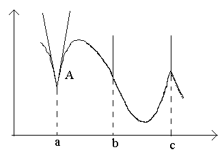
Consider the points in the figure a, b, c.
At the point a at Δ x→0 the relation has no limit (because the one-sided limits are different for Δ x→0–0 and Δ x→0+0). At the point A the graph has no defined tangent, but there are two different one-sided tangents with slopes To 1 and To 2. This type of point is called a corner point.
At the point b at Δ x→0 the ratio is of constant sign infinitely large value . The function has an infinite derivative. At this point, the graph has a vertical tangent. Point type - "inflection point" with a vertical tangent.
At the point c one-sided derivatives are infinitely large quantities of different signs. At this point, the graph has two merged vertical tangents. Type - "cusp" with a vertical tangent - a special case of a corner point.

Definition. If the function f(x) is defined on the interval [ a, b], is continuous at every point of the interval ( a, b), at the point a continuous on the right, at a point b is continuous on the left, then we say that the function f(x) continuous on the segment [a, b].
In other words, the function f(x) is continuous on the interval [ a, b] if three conditions are met:
1) "x 0 Î( a, b): f(x) = f(x 0);
2) f(x) = f(a);
3) f(x) = f(b).
For functions that are continuous on an interval, we consider some properties, which we formulate in the form of the following theorems without proofs.
Theorem 1. If the function f(x) is continuous on the interval [ a, b], then it reaches its smallest and its largest value on this segment.
This theorem states (Fig. 1.15) that on the segment [ a, b] there is such a point x 1 that f(x 1) £ f(x) for any x from [ a, b] and that there is a point x 2 (x 2 О[ a, b]) such that " xÎ[ a, b] (f(x 2) ³ f(x)).
Meaning f(x 1) is the largest for the given function on [ a, b], a f(x 2) - the smallest. Denote: f(x 1) = M, f(x 2) =m. Since for f(x) the following inequality holds: " xÎ[ a, b] m£ f(x) £ M, then we obtain the following corollary from Theorem 1.
Consequence. If the function f(x) is continuous on a segment, then it is bounded on this segment.
Theorem 2. If the function f(x) is continuous on the interval [ a,b] and takes on values of different signs at the ends of the segment, then there is such an interior point x 0 segment [ a, b], in which the function turns to 0, i.e. $ x 0 Î ( a, b) (f(x 0) = 0).
This theorem states that the graph of a function y=f(x), continuous on the interval [ a, b], crosses the axis Ox at least once if the values f(a) and f(b) have opposite signs. So, (Fig. 1.16) f(a) > 0, f(b) < 0 и функция f(x) vanishes at points x 1 , x 2 , x 3 .
Theorem 3. Let the function f(x) is continuous on the interval [ a, b], f(a) = A, f(b) = B and A¹ B. (Fig. 1.17). Then for any number C, concluded between the numbers A and B, there is such an interior point x 0 segment [ a, b], what f(x 0) = C.
Consequence. If the function f(x) is continuous on the interval [ a, b], m- the smallest value f(x), M- the largest value of the function f(x) on the segment [ a, b], then the function takes (at least once) any value m between m and M, and therefore the segment [ m, M] is the set of all values of the function f(x) on the segment [ a, b].
Note that if the function is continuous on the interval ( a, b) or has on the interval [ a, b] of the discontinuity point, then Theorems 1, 2, 3 cease to be true for such a function.
In conclusion, consider the theorem on the existence of an inverse function.
Recall that an interval is a segment, an interval, or a finite or infinite half-interval.
 |
Theorem 4. Let f(x) is continuous on the interval X, increases (or decreases) by X and has a range of values Y. Then for the function y=f(x) there is an inverse function x= j(y) defined on the interval Y, continuous and increasing (or decreasing) on Y with many meanings X.
Comment. Let the function x= j(y) is inverse for the function f(x). Since the argument is usually denoted by x, and the function through y, then we write inverse function as y=j(x).
Example 1. Function y=x 2 (Fig. 1.8, a) on the set X= }