Homogeneous equation of the first order. Homogeneous differential equations

Ready-made answers to examples for homogeneous differential equations Many students are looking for the first order (DEs of the 1st order are the most common in training), then you can analyze them in detail. But before proceeding to the consideration of examples, we recommend that you carefully read a brief theoretical material.
Equations of the form P(x,y)dx+Q(x,y)dy=0, where the functions P(x,y) and Q(x,y) are homogeneous functions of the same order, are called homogeneous differential equation(ODR).

Scheme for solving a homogeneous differential equation

1. First you need to apply the substitution y=z*x , where z=z(x) is a new unknown function (thus the original equation is reduced to a differential equation with separable variables.
2. The derivative of the product is y"=(z*x)"=z"*x+z*x"=z"*x+z or in differentials dy=d(zx)=z*dx+x*dz.
3. Next, we substitute the new function y and its derivative y "(or dy) into DE with separable variables with respect to x and z .
4. Having solved the differential equation with separable variables, we will make an inverse replacement y=z*x, therefore z= y/x, and we get common decision(general integral) of the differential equation.
5. If the initial condition y(x 0)=y 0 is given, then we find a particular solution to the Cauchy problem. In theory, everything sounds easy, but in practice, not everyone is so fun to solve differential equations. Therefore, to deepen knowledge, consider common examples. On easy tasks, there is not much to teach you, so we will immediately move on to more complex ones.

Calculations of homogeneous differential equations of the first order

Example 1

Solution: Divide right side equations for a variable that is a factor near the derivative. As a result, we arrive at homogeneous differential equation of order 0

And here it became interesting to many, how to determine the order of a function of a homogeneous equation?
The question is relevant enough, and the answer to it is as follows:
on the right side, we substitute the value t*x, t*y instead of the function and the argument. When simplifying, the parameter "t" is obtained to a certain degree k, and it is called the order of the equation. In our case, "t" will be reduced, which is equivalent to the 0th degree or zero order of the homogeneous equation.
Further on the right side we can move on to the new variable y=zx; z=y/x .
At the same time, do not forget to express the derivative of "y" through the derivative of the new variable. By the rule of parts, we find

Equations in Differentials will take the form

We reduce the joint terms on the right and left sides and pass to differential equation with separated variables.

Let us integrate both parts of the DE

For the convenience of further transformations, we immediately introduce the constant under the logarithm

According to the properties of logarithms, the obtained logarithmic equation is equivalent to the following

This entry is not yet a solution (answer), you need to return to the change of variables performed

Thus they find general solution of differential equations. If you carefully read the previous lessons, then we said that you should be able to apply the scheme for calculating equations with separated variables freely and such equations will have to be calculated for more complex types of remote control.

Example 2 Find the integral of a differential equation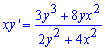

Solution: The scheme for calculating homogeneous and summary DEs is now familiar to you. We transfer the variable to the right side of the equation, and also in the numerator and denominator we take out x 2 as a common factor

Thus, we obtain a homogeneous zero-order DE.
The next step is to introduce the change of variables z=y/x, y=z*x , which we will constantly remind you to memorize

After that, we write the DE in differentials

Next, we transform the dependence to differential equation with separated variables

and solve it by integration.

The integrals are simple, the rest of the transformations are based on the properties of the logarithm. The last action involves exposing the logarithm. Finally, we return to the original replacement and write in the form

The constant "C" takes any value. All those who study in absentia have problems in exams with this type of equations, so please carefully look at and remember the calculation scheme.

Example 3 Solve differential equation

Solution: As follows from the above technique, differential equations of this type solve by introducing a new variable. Let's rewrite the dependence so that the derivative is without a variable

Further, by analyzing the right side, we see that the part -ee is present everywhere and denoted by the new unknown
z=y/x, y=z*x .
Finding the derivative of y

Taking into account the replacement, we rewrite the original DE in the form

Simplify the same terms, and reduce all received terms to DE with separated variables

By integrating both sides of the equality

we come to the solution in the form of logarithms

By exposing the dependencies we find general solution of a differential equation

which, after substituting the initial change of variables into it, takes the form

Here C is a constant, which can be extended from the Cauchy condition. If the Cauchy problem is not given, then it becomes an arbitrary real value.
That's all the wisdom in the calculus of homogeneous differential equations.

I think we should start with the history of such a glorious mathematical tool as differential equations. Like all differential and integral calculus, these equations were invented by Newton at the end of the 17th century. He considered this very discovery of his so important that he even encrypted the message, which today can be translated something like this: "All laws of nature are described by differential equations." This may seem like an exaggeration, but it's true. Any law of physics, chemistry, biology can be described by these equations.

A huge contribution to the development and creation of the theory of differential equations was made by the mathematicians Euler and Lagrange. Already in the 18th century, they discovered and developed what they are now studying in the senior courses of universities.

A new milestone in the study of differential equations began thanks to Henri Poincare. He created a "qualitative theory of differential equations", which, in combination with the theory of functions of a complex variable, made a significant contribution to the foundation of topology - the science of space and its properties.

What are differential equations?

Many people are afraid of one phrase. However, in this article we will detail the whole essence of this very useful mathematical apparatus, which is actually not as complicated as it seems from the name. In order to start talking about first-order differential equations, you should first get acquainted with the basic concepts that are inherently related to this definition. Let's start with the differential.

Differential

Many people know this concept from school. However, let's take a closer look at it. Imagine a graph of a function. We can increase it to such an extent that any of its segments will take the form of a straight line. On it we take two points that are infinitely close to each other. The difference between their coordinates (x or y) will be an infinitesimal value. It is called a differential and is denoted by the signs dy (differential from y) and dx (differential from x). It is very important to understand that the differential is not a finite value, and this is its meaning and main function.

And now it is necessary to consider the following element, which will be useful to us in explaining the concept of a differential equation. This is a derivative.

Derivative

We all probably heard this concept in school. The derivative is said to be the rate of growth or decrease of a function. However, much of this definition becomes incomprehensible. Let's try to explain the derivative in terms of differentials. Let's go back to an infinitesimal segment of a function with two points that are at a minimum distance from each other. But even for this distance, the function manages to change by some amount. And in order to describe this change, they came up with a derivative, which can otherwise be written as a ratio of differentials: f (x) "=df / dx.

Now it is worth considering the basic properties of the derivative. There are only three of them:

1. The derivative of the sum or difference can be represented as the sum or difference of the derivatives: (a+b)"=a"+b" and (a-b)"=a"-b".
2. The second property is related to multiplication. The derivative of a product is the sum of the products of one function and the derivative of another: (a*b)"=a"*b+a*b".
3. The derivative of the difference can be written as the following equality: (a/b)"=(a"*b-a*b")/b 2 .

All these properties will be useful to us for finding solutions to first-order differential equations.

There are also partial derivatives. Let's say we have a function z that depends on variables x and y. To calculate the partial derivative of this function, say, with respect to x, we need to take the variable y as a constant and simply differentiate.

Integral

Other important concept- integral. In fact, this is the direct opposite of the derivative. There are several types of integrals, but to solve the simplest differential equations, we need the most trivial

So, Let's say we have some dependency of f on x. We take the integral from it and get the function F (x) (often called the antiderivative), the derivative of which is equal to the original function. Thus F(x)"=f(x). It also follows that the integral of the derivative is equal to the original function.

When solving differential equations, it is very important to understand the meaning and function of the integral, since you will have to take them very often to find a solution.

Equations are different depending on their nature. In the next section, we will consider the types of first-order differential equations, and then we will learn how to solve them.

Classes of differential equations

"Diffura" are divided according to the order of the derivatives involved in them. Thus, there is the first, second, third and more order. They can also be divided into several classes: ordinary and partial derivatives.

In this article, we will consider ordinary differential equations of the first order. We will also discuss examples and ways to solve them in the following sections. We will consider only ODEs, because these are the most common types of equations. Ordinary are divided into subspecies: with separable variables, homogeneous and heterogeneous. Next, you will learn how they differ from each other, and learn how to solve them.

In addition, these equations can be combined, so that after we get a system of differential equations of the first order. We will also consider such systems and learn how to solve them.

Why are we considering only the first order? Because you need to start with a simple one, and it is simply impossible to describe everything related to differential equations in one article.

Separable Variable Equations

These are perhaps the simplest first-order differential equations. These include examples that can be written like this: y "=f (x) * f (y). To solve this equation, we need a formula for representing the derivative as a ratio of differentials: y" = dy / dx. Using it, we get the following equation: dy/dx=f(x)*f(y). Now we can turn to the method for solving standard examples: we will divide the variables into parts, that is, we will transfer everything with the y variable to the part where dy is located, and we will do the same with the x variable. We obtain an equation of the form: dy/f(y)=f(x)dx, which is solved by taking the integrals of both parts. Do not forget about the constant, which must be set after taking the integral.

The solution of any "diffurance" is a function of the dependence of x on y (in our case) or, if there is a numerical condition, then the answer is in the form of a number. Let's take a look at specific example the whole course of the solution:

We transfer variables in different directions:

Now we take integrals. All of them can be found in a special table of integrals. And we get:

log(y) = -2*cos(x) + C

If required, we can express "y" as a function of "x". Now we can say that our differential equation is solved if no condition is given. A condition can be given, for example, y(n/2)=e. Then we simply substitute the value of these variables into the solution and find the value of the constant. In our example, it is equal to 1.

Homogeneous differential equations of the first order

Now let's move on to the more difficult part. Homogeneous differential equations of the first order can be written in general view so: y"=z(x,y). It should be noted that the right function of two variables is homogeneous, and it cannot be divided into two dependencies: z on x and z on y. Checking whether the equation is homogeneous or not is quite simple : we make the replacement x=k*x and y=k*y.Now we cancel all k.If all these letters have been reduced, then the equation is homogeneous and you can safely proceed to solve it.Looking ahead, let's say: the principle of solving these examples is also very simple .

We need to make a replacement: y=t(x)*x, where t is some function that also depends on x. Then we can express the derivative: y"=t"(x)*x+t. Substituting all this into our original equation and simplifying it, we get an example with separable variables t and x. We solve it and get the dependence t(x). When we got it, we simply substitute y=t(x)*x into our previous replacement. Then we get the dependence of y on x.

To make it clearer, let's look at an example: x*y"=y-x*e y/x .

When checking with a replacement, everything is reduced. So the equation is really homogeneous. Now we make another replacement that we talked about: y=t(x)*x and y"=t"(x)*x+t(x). After simplification, we get the following equation: t "(x) * x \u003d -et. We solve the resulting example with separated variables and get: e -t \u003d ln (C * x). We only need to replace t with y / x (because if y \u003d t * x, then t \u003d y / x), and we get the answer: e -y / x \u003d ln (x * C).

Linear differential equations of the first order

It's time to consider another broad topic. We will analyze inhomogeneous differential equations of the first order. How are they different from the previous two? Let's figure it out. Linear differential equations of the first order in general form can be written as follows: y " + g (x) * y \u003d z (x). It is worth clarifying that z (x) and g (x) can be constant values.

And now an example: y" - y*x=x 2 .

There are two ways to solve, and we will analyze both in order. The first one is the method of variation of arbitrary constants.

In order to solve the equation in this way, you must first equate the right side to zero and solve the resulting equation, which, after transferring the parts, will take the form:

ln|y|=x 2 /2 + C;

y \u003d e x2 / 2 * y C \u003d C 1 * e x2 / 2.

Now we need to replace the constant C 1 with the function v(x), which we have to find.

Let's change the derivative:

y"=v"*e x2/2 -x*v*e x2/2 .

Let's substitute these expressions into the original equation:

v"*e x2/2 - x*v*e x2/2 + x*v*e x2/2 = x 2 .

It can be seen that two terms are canceled on the left side. If in some example this did not happen, then you did something wrong. Let's continue:

v"*e x2/2 = x 2 .

Now we solve the usual equation in which we need to separate the variables:

dv/dx=x 2 /e x2/2 ;

dv = x 2 *e - x2/2 dx.

To extract the integral, we have to apply integration by parts here. However, this is not the topic of our article. If you are interested, you can learn how to perform such actions yourself. It is not difficult, and with sufficient skill and care, it does not take much time.

Let us turn to the second method for solving inhomogeneous equations: the Bernoulli method. Which approach is faster and easier is up to you.

So, when solving the equation by this method, we need to make a replacement: y=k*n. Here k and n are some x-dependent functions. Then the derivative will look like this: y"=k"*n+k*n". We substitute both replacements into the equation:

k"*n+k*n"+x*k*n=x 2 .

Grouping:

k"*n+k*(n"+x*n)=x 2 .

Now we need to equate to zero what is in brackets. Now, if we combine the two resulting equations, we get a system of first-order differential equations that needs to be solved:

We solve the first equality as an ordinary equation. To do this, you need to separate the variables:

We take the integral and get: ln(n)=x 2 /2. Then, if we express n:

Now we substitute the resulting equality into the second equation of the system:

k "*e x2/2 \u003d x 2.

And transforming, we get the same equality as in the first method:

dk=x 2 /e x2/2 .

We will also not analyze further actions. It is worth saying that at first the solution of first-order differential equations causes significant difficulties. However, with a deeper immersion in the topic, it starts to get better and better.

Where are differential equations used?

Differential equations are very actively used in physics, since almost all the basic laws are written in differential form, and the formulas that we see are the solution of these equations. In chemistry, they are used for the same reason: basic laws are derived from them. In biology, differential equations are used to model the behavior of systems, such as predator-prey. They can also be used to create reproduction models of, say, a colony of microorganisms.

How will differential equations help in life?

The answer to this question is simple: no way. If you are not a scientist or engineer, then they are unlikely to be useful to you. However, for general development It does not hurt to know what a differential equation is and how it is solved. And then the question of a son or daughter "what is a differential equation?" won't confuse you. Well, if you are a scientist or an engineer, then you yourself understand the importance of this topic in any science. But the most important thing is that now the question "how to solve a first-order differential equation?" you can always answer. Agree, it's always nice when you understand what people are even afraid to understand.

Main problems in learning

The main problem in understanding this topic is the poor skill of integrating and differentiating functions. If you are bad at taking derivatives and integrals, then you should probably learn more, master different methods integration and differentiation, and only then proceed to the study of the material that was described in the article.

Some people are surprised when they learn that dx can be transferred, because earlier (in school) it was stated that the fraction dy / dx is indivisible. Here you need to read the literature on the derivative and understand that it is the ratio of infinitesimal quantities that can be manipulated when solving equations.

Many do not immediately realize that the solution of first-order differential equations is often a function or an integral that cannot be taken, and this delusion gives them a lot of trouble.

What else can be studied for a better understanding?

It is best to start further immersion in the world of differential calculus with specialized textbooks, for example, mathematical analysis for students of non-mathematical specialties. Then you can move on to more specialized literature.

It is worth saying that, in addition to differential equations, there are also integral equations, so you will always have something to strive for and something to study.

Conclusion

We hope that after reading this article you have an idea of ​​what differential equations are and how to solve them correctly.

In any case, mathematics is somehow useful to us in life. It develops logic and attention, without which every person is like without hands.

In some problems of physics, a direct connection between the quantities describing the process cannot be established. But there is a possibility to obtain an equality containing the derivatives of the functions under study. This is how differential equations arise and the need to solve them in order to find an unknown function.

This article is intended for those who are faced with the problem of solving a differential equation in which the unknown function is a function of one variable. The theory is built in such a way that with a zero understanding of differential equations, you can do your job.

Each type of differential equations is associated with a solution method with detailed explanations and solutions of typical examples and problems. You just have to determine the type of differential equation of your problem, find a similar analyzed example and carry out similar actions.

To successfully solve differential equations on your part, you will also need the ability to find sets of antiderivatives ( indefinite integrals) various functions. If necessary, we recommend that you refer to the section.

First, we consider the types of ordinary differential equations of the first order that can be solved with respect to the derivative, then we move on to second-order ODEs, then we dwell on higher-order equations and finish with systems of differential equations.

Recall that if y is a function of the argument x .

First order differential equations.

The simplest differential equations of the first order of the form .

Let us write down several examples of such DE .

Differential Equations can be resolved with respect to the derivative by dividing both sides of the equality by f(x) . In this case, we arrive at the equation , which will be equivalent to the original one for f(x) ≠ 0 . Examples of such ODEs are .

If there are values ​​of the argument x for which the functions f(x) and g(x) simultaneously vanish, then additional solutions appear. Additional solutions to the equation given x are any functions defined for those argument values. Examples of such differential equations are .

Second order differential equations.

Second Order Linear Homogeneous Differential Equations with Constant Coefficients.

LODE with constant coefficients is a very common type of differential equations. Their solution is not particularly difficult. First, the roots of the characteristic equation are found . For different p and q, three cases are possible: the roots of the characteristic equation can be real and different, real and coinciding or complex conjugate. Depending on the values ​​of the roots of the characteristic equation, the general solution of the differential equation is written as , or , or respectively.

For example, consider a second-order linear homogeneous differential equation with constant coefficients. The roots of his characteristic equation are k 1 = -3 and k 2 = 0. The roots are real and different, therefore, the general solution to the LDE with constant coefficients is


Linear Nonhomogeneous Second Order Differential Equations with Constant Coefficients.

The general solution of the second-order LIDE with constant coefficients y is sought as the sum of the general solution of the corresponding LODE and a particular solution of the original inhomogeneous equation, that is, . The previous paragraph is devoted to finding a general solution to a homogeneous differential equation with constant coefficients. And a particular solution is determined either by the method of indefinite coefficients at certain form function f(x) , standing on the right side of the original equation, or by the method of variation of arbitrary constants.

As examples of second-order LIDEs with constant coefficients, we present


To understand the theory and get acquainted with the detailed solutions of examples, we offer you on the page linear inhomogeneous differential equations of the second order with constant coefficients.

Linear Homogeneous Differential Equations (LODEs) and second-order linear inhomogeneous differential equations (LNDEs).

A special case of differential equations of this type are LODE and LODE with constant coefficients.

The general solution of the LODE on a certain interval is represented by a linear combination of two linearly independent particular solutions y 1 and y 2 of this equation, that is, .

The main difficulty lies precisely in finding linearly independent partial solutions of this type of differential equation. Usually, particular solutions are chosen from the following systems of linearly independent functions:


However, particular solutions are not always presented in this form.

An example of a LODU is .

The general solution of the LIDE is sought in the form , where is the general solution of the corresponding LODE, and is a particular solution of the original differential equation. We just talked about finding, but it can be determined using the method of variation of arbitrary constants.

An example of an LNDE is .

Higher order differential equations.

Differential equations admitting order reduction.

Order of differential equation , which does not contain the desired function and its derivatives up to k-1 order, can be reduced to n-k by replacing .

In this case , and the original differential equation reduces to . After finding its solution p(x), it remains to return to the replacement and determine the unknown function y .

For example, the differential equation after the replacement becomes a separable equation , and its order is reduced from the third to the first.

For example, the function
is a homogeneous function of the first dimension, since

is a homogeneous function of the third dimension, since

is a homogeneous function of the zero dimension, since

, i.e.
.

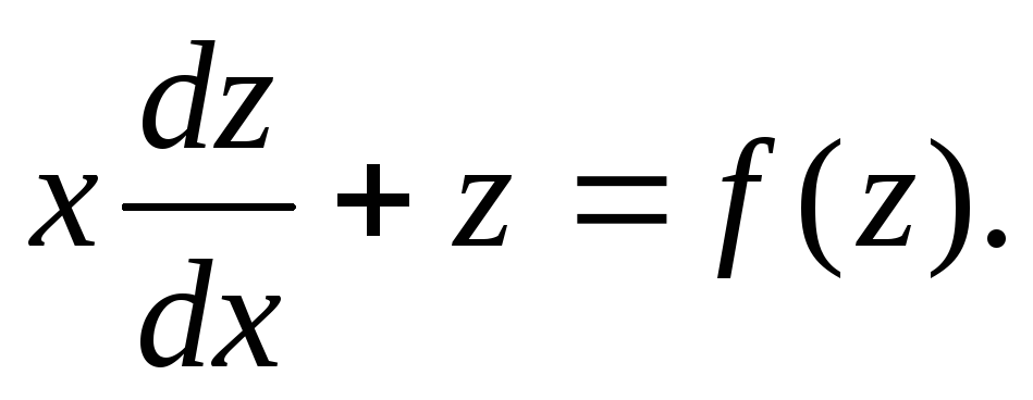
Definition 2. First order differential equation y" = f(x, y) is called homogeneous if the function f(x, y) is a homogeneous zero dimension function with respect to x and y, or, as they say, f(x, y) is a homogeneous function of degree zero.

It can be represented as

which allows us to define a homogeneous equation as a differential equation that can be transformed to the form (3.3).

Replacement
reduces a homogeneous equation to an equation with separable variables. Indeed, after substitution y=xz we get
,
Separating the variables and integrating, we find:

,

Example 1. Solve the equation.

Δ We assume y=zx,
We substitute these expressions y and dy into this equation:
or
Separating variables:
and integrate:
,

Replacing z on the , we get
.

Example 2 Find the general solution of the equation.

Δ In this equation P (x,y) =x 2 -2y 2 ,Q(x,y) =2xy are homogeneous functions of the second dimension, therefore, this equation is homogeneous. It can be represented as
and solve in the same way as above. But we use a different notation. Let's put y = zx, where dy = zdx + xdz. Substituting these expressions into the original equation, we will have

dx+2 zxdz = 0 .

We separate the variables, counting

.

We integrate term by term this equation

, where

that is
. Returning to the old function
find a general solution


Example 3 . Find a general solution to the equation
.

Δ Chain of transformations: ,y = zx,
,
,
,
,
,
,
,
, ,
. 

Lecture 8

4. Linear differential equations of the first order A linear differential equation of the first order has the form

Here, is the free term, also called the right side of the equation. In this form, we will consider the linear equation in what follows.

If
0, then equation (4.1a) is called linear inhomogeneous. If
0, then the equation takes the form

and is called linear homogeneous.

The name of equation (4.1a) is explained by the fact that the unknown function y and its derivative enter it linearly, i.e. in the first degree.

In a linear homogeneous equation, the variables are separated. Rewriting it in the form
where
and integrating, we get:
,those.

When divided by we lose the decision
. However, it can be included in the found family of solutions (4.3) if we assume that WITH can also take the value 0.

There are several methods for solving equation (4.1a). According to Bernoulli method, the solution is sought as a product of two functions of X:

One of these functions can be chosen arbitrarily, since only the product UV must satisfy the original equation, the other is determined on the basis of equation (4.1a).

Differentiating both sides of equality (4.4), we find
.

Substituting the resulting derivative expression , as well as the value at into equation (4.1a), we obtain
, or

those. as a function v take the solution of the homogeneous linear equation (4.6):

(Here C it is obligatory to write, otherwise you will get not a general, but a particular solution).

Thus, we see that as a result of the substitution (4.4) used, equation (4.1a) reduces to two equations with separable variables (4.6) and (4.7).

Substituting
and v(x) into formula (4.4), we finally obtain

,

.

Example 1 Find a general solution to the equation

 We put
, then
. Substituting Expressions and into the original equation, we get
or
(*)

We equate to zero the coefficient at :

Separating the variables in the resulting equation, we have


(arbitrary constant C do not write), hence v= x. Found value v substitute into the equation (*):

,
,
.

Hence,
general solution of the original equation.

Note that the equation (*) could be written in an equivalent form:

.

Randomly choosing a function u, but not v, we could assume
. This way of solving differs from the considered one only by replacing v on the u(and therefore u on the v), so that the final value at turns out to be the same.

Based on the above, we obtain an algorithm for solving a first-order linear differential equation.

Note further that sometimes a first-order equation becomes linear if at be considered an independent variable, and x- dependent, i.e. change roles x and y. This can be done provided that x and dx enter the equation linearly.

Example 2 . solve the equation
.

In appearance, this equation is not linear with respect to the function at.

However, if we consider x as a function of at, then, given that
, it can be brought to the form

(4.1 b)

Replacing on the , we get
or
. Dividing both sides of the last equation by the product ydy, bring it to the form

, or
. (**)

Here P(y)=,
. This is a linear equation with respect to x. We believe
,
. Substituting these expressions into (**), we get

or
.

We choose v so that
,
, where
;
. Then we have
,
,
.

Because
, then we arrive at the general solution of this equation in the form

.

Note that in equation (4.1a) P(x) and Q (x) can occur not only as functions of x, but also constants: P= a,Q= b. Linear Equation

can also be solved using the substitution y= UV and separation of variables:

;
.

From here
;
;
; where
. Getting rid of the logarithm, we obtain the general solution of the equation

(here
).

At b= 0 we come to the solution of the equation

(see exponential growth equation (2.4) for
).

First, we integrate the corresponding homogeneous equation (4.2). As indicated above, its solution has the form (4.3). We will consider the factor WITH in (4.3) by a function of X, i.e. essentially making a change of variable

whence, integrating, we find

Note that, according to (4.14) (see also (4.9)), the general solution of the inhomogeneous linear equation is equal to the sum of the general solution of the corresponding homogeneous equation (4.3) and the particular solution of the inhomogeneous equation determined by the second term in (4.14) (and in ( 4.9)).

When solving specific equations, one should repeat the above calculations, and not use the cumbersome formula (4.14).

We apply the Lagrange method to the equation considered in example 1 :

.

We integrate the corresponding homogeneous equation
.

Separating the variables, we get
and beyond
. Solving an expression by a formula y = Cx. The solution of the original equation is sought in the form y = C(x)x. Substituting this expression into the given equation, we obtain
;
;
,
. The general solution of the original equation has the form

.

In conclusion, we note that the Bernoulli equation is reduced to a linear equation

, ( )

which can be written as

.

replacement
it is reduced to a linear equation:

,
,
.

The Bernoulli equations are also solved by the methods described above.

Example 3 . Find a general solution to the equation
.

 Chain of transformations:
,
,,
,
,
,
,
,
,
,
,
,
,
,


The function f(x,y) is called homogeneous function of their dimension arguments n if the identity f(tx,ty) \equiv t^nf(x,y).

For example, the function f(x,y)=x^2+y^2-xy is a homogeneous function of the second dimension, since

F(tx,ty)=(tx)^2+(ty)^2-(tx)(ty)=t^2(x^2+y^2-xy)=t^2f(x,y).

For n=0 we have a zero dimension function. For instance, \frac(x^2-y^2)(x^2+y^2) is a homogeneous zero dimension function, since

(f(tx,ty)=\frac((tx)^2-(ty)^2)((tx)^2+(ty)^2)=\frac(t^2(x^2-y^ 2))(t^2(x^2+y^2))=\frac(x^2-y^2)(x^2+y^2)=f(x,y).)

Differential equation of the form \frac(dy)(dx)=f(x,y) is said to be homogeneous with respect to x and y if f(x,y) is a homogeneous function of its null dimension arguments. A homogeneous equation can always be represented as

\frac(dy)(dx)=\varphi\!\left(\frac(y)(x)\right).

By introducing a new desired function u=\frac(y)(x) , equation (1) can be reduced to an equation with separating variables:

X\frac(du)(dx)=\varphi(u)-u.

If u=u_0 is the root of the equation \varphi(u)-u=0 , then the solution to the homogeneous equation will be u=u_0 or y=u_0x (the straight line passing through the origin).

Comment. When solving homogeneous equations, it is not necessary to reduce them to the form (1). You can immediately do the substitution y=ux .

Example 1 Solve a homogeneous equation xy"=\sqrt(x^2-y^2)+y.

Solution. We write the equation in the form y"=\sqrt(1-(\left(\frac(y)(x)\right)\^2}+\frac{y}{x} !} so the given equation turns out to be homogeneous with respect to x and y. Let's put u=\frac(y)(x) , or y=ux . Then y"=xu"+u . Substituting expressions for y and y" into the equation, we get x\frac(du)(dx)=\sqrt(1-u^2). Separating variables: \frac(du)(1-u^2)=\frac(dx)(x). From here, by integration, we find

\arcsin(u)=\ln|x|+\ln(C_1)~(C_1>0), or \arcsin(u)=\ln(C_1|x|).

Since C_1|x|=\pm(C_1x) , denoting \pm(C_1)=C , we get \arcsin(u)=\ln(Cx), where |\ln(Cx)|\leqslant\frac(\pi)(2) or e^(-\pi/2)\leqslant(Cx)\leqslant(e^(\pi/2)). Replacing u with \frac(y)(x) , we will have the general integral \arcsin(y)(x)=\ln(Cx).

Hence the general solution: y=x\sin\ln(Cx) .

When separating variables, we divided both sides of the equation by the product x\sqrt(1-u^2) , so we could lose the solution that turns this product to zero.

Let's now put x=0 and \sqrt(1-u^2)=0 . But x\ne0 due to the substitution u=\frac(y)(x) , and from the relation \sqrt(1-u^2)=0 we get that 1-\frac(y^2)(x^2)=0, whence y=\pm(x) . By direct verification, we make sure that the functions y=-x and y=x are also solutions to this equation.

Example 2 Consider the family of integral curves C_\alpha of the homogeneous equation y"=\varphi\!\left(\frac(y)(x)\right). Show that the tangents at the corresponding points to the curves defined by this homogeneous differential equation are parallel to each other.

Note: We will call relevant those points on the C_\alpha curves that lie on the same ray starting from the origin.

Solution. By definition of the corresponding points, we have \frac(y)(x)=\frac(y_1)(x_1), so that, by virtue of the equation itself, y"=y"_1, where y" and y"_1 are the slopes of the tangents to the integral curves C_\alpha and C_(\alpha_1) , at the points M and M_1, respectively (Fig. 12).

Equations Reducing to Homogeneous

A. Consider a differential equation of the form

\frac(dy)(dx)=f\!\left(\frac(ax+by+c)(a_1x+b_1y+c_1)\right).

where a,b,c,a_1,b_1,c_1 are constants and f(u) is continuous function of its argument u .

If c=c_1=0 , then equation (3) is homogeneous and it integrates as above.

If at least one of the numbers c,c_1 is different from zero, then two cases should be distinguished.

1) Determinant \Delta=\begin(vmatrix)a&b\\a_1&b_1\end(vmatrix)\ne0. Introducing new variables \xi and \eta according to the formulas x=\xi+h,~y=\eta+k , where h and k are still undefined constants, we bring equation (3) to the form

\frac(d\eta)(d\xi)=f\!\left(\frac(a\xi+b\eta+ah+bk+c)(a_1\xi+b_2\eta+a_1h+b_1k+c_1 )\right).

Choosing h and k as a solution to the system linear equations

\begin(cases)ah+bk+c=0,\\a_1h+b_1k+c_1=0\end(cases)~(\Delta\ne0),

we obtain a homogeneous equation \frac(d\eta)(d\xi)=f\!\left(\frac(a\xi+b\eta)(a_1\xi+b_1\eta)\right). Having found its general integral and replacing \xi with x-h in it, and \eta with y-k , we obtain the general integral of equation (3).

2) Determinant \Delta=\begin(vmatrix)a&b\\a_1&b_1\end(vmatrix)=0. System (4) has no solutions in the general case, and the above method is not applicable; in this case \frac(a_1)(a)=\frac(b_1)(b)=\lambda, and, therefore, equation (3) has the form \frac(dy)(dx)=f\!\left(\frac(ax+by+c)(\lambda(ax+by)+c_1)\right). The substitution z=ax+by brings it to a separable variable equation.

Example 3 solve the equation (x+y-2)\,dx+(x-y+4)\,dy=0.

Solution. Consider a system of linear algebraic equations \begin(cases)x+y-2=0,\\x-y+4=0.\end(cases)

The determinant of this system \Delta=\begin(vmatrix)\hfill1&\hfill1\\\hfill1&\hfill-1\end(vmatrix)=-2\ne0.

The system has only decision x_0=-1,~y_0=3 . We make the replacement x=\xi-1,~y=\eta+3 . Then equation (5) takes the form

(\xi+\eta)\,d\xi+(\xi-\eta)\,d\eta=0.

This equation is a homogeneous equation. Setting \eta=u\xi , we get

(\xi+\xi(u))\,d\xi+(\xi-\xi(u))(\xi\,du+u\,d\xi)=0, where (1+2u-u^2)\,d\xi+\xi(1-u)\,du=0.

Separating Variables \frac(d\xi)(\xi)+\frac(1-u)(1+2u-u^2)\,du=0.

Integrating, we find \ln|\xi|+\frac(1)(2)\ln|1+2u-u^2|=\ln(C) or \xi^2(1+2u-u^2)=C .

Returning to the variables x,~y :

(x+1)^2\left=C_1 or x^2+2xy-y^2-4x+8y=C~~(C=C_1+14).

Example 4 solve the equation (x+y+1)\,dx+(2x+2y-1)\,dy=0.

Solution. System of linear algebraic equations \begin(cases)x+y+1=0,\\2x+2y-1=0\end(cases) incompatible. In this case, the method applied in the previous example is not suitable. To integrate the equation, we use the substitution x+y=z , dy=dz-dx . The equation will take the form

(2-z)\,dx+(2z-1)\,dz=0.

Separating the variables, we get

Dx-\frac(2z-1)(z-2)\,dz=0 hence x-2z-3\ln|z-2|=C.

Returning to the variables x,~y , we obtain the general integral of this equation

X+2y+3\ln|x+y-2|=C.

B. Sometimes the equation can be reduced to a homogeneous one by changing the variable y=z^\alpha . This is the case when all terms in the equation are of the same dimension, if the variable x is given the dimension 1, the variable y is given the dimension \alpha, and the derivative \frac(dy)(dx) is given the dimension \alpha-1 .

Example 5 solve the equation (x^2y^2-1)\,dy+2xy^3\,dx=0.

Solution. Making a substitution y=z^\alpha,~dy=\alpha(z^(\alpha-1))\,dz, where \alpha is an arbitrary number for now, which we will choose later. Substituting expressions for y and dy into the equation, we get

\alpha(x^2x^(2\alpha)-1)z^(\alpha-1)\,dz+2xz^(3\alpha)\,dx=0 or \alpha(x^2z^(3\alpha-1)-z^(\alpha-1))\,dz+2xz^(3\alpha)\,dx=0,

Note that x^2z^(3\alpha-1) has the dimension 2+3\alpha-1=3\alpha+1, z^(\alpha-1) has dimension \alpha-1 , xz^(3\alpha) has dimension 1+3\alpha . The resulting equation will be homogeneous if the measurements of all terms are the same, i.e. if the condition is met 3\alpha+1=\alpha-1, or \alpha-1 .

Let's put y=\frac(1)(z) ; the original equation takes the form

\left(\frac(1)(z^2)-\frac(x^2)(z^4)\right)dz+\frac(2x)(z^3)\,dx=0 or (z^2-x^2)\,dz+2xz\,dx=0.

Let's put now z=ux,~dz=u\,dx+x\,du. Then this equation will take the form (u^2-1)(u\,dx+x\,du)+2u\,dx=0, where u(u^2+1)\,dx+x(u^2-1)\,du=0.

Separating the variables in this equation \frac(dx)(x)+\frac(u^2-1)(u^3+u)\,du=0. Integrating, we find

\ln|x|+\ln(u^2+1)-\ln|u|=\ln(C) or \frac(x(u^2+1))(u)=C.

Replacing u with \frac(1)(xy) , we get the general integral of this equation 1+x^2y^2=Cy.

The equation has another obvious solution y=0 , which is obtained from common integral for C\to\infty , if the integral is written as y=\frac(1+x^2y^2)(C), and then jump to the limit at C\to\infty . Thus, the function y=0 is a particular solution to the original equation.

Javascript is disabled in your browser.
ActiveX controls must be enabled in order to make calculations!